Example
This example code is base on an exisiting tutorial made available by Sinabs. It is adapted in order to work with VLab.
It shows how to define a standard CNN model, load a NMNIST dataset from Tonic, train the model, convert it to SNN, validate its accuracy and save it as a file. Convert that Tonic dataset into the format expected by the Speck and save it as a file. Run the benchmarking using the dAIEdgeVlab Python Client, get the output results, analyse the spiking activity, the power consumption and calculate the accuracy.
Create the CNN model
Speck™ constraints the model architecture and operations.
from torch import nn

# Define a CNN model
cnn = nn.Sequential(
    # [2,34,34] -> [8, 17 ,17]
    nn.Conv2d(in_channels=2, out_channels=8, kernel_size=(3,3), padding=(1,1), bias=False),
    nn.ReLU(),
    nn.AvgPool2d(2,2),
    # [8,17,17] -> [16,8,8]
    nn.Conv2d(in_channels=8, out_channels=16, kernel_size=(3,3), padding=(1,1), bias=False),
    nn.ReLU(),
    nn.AvgPool2d(2,2),
    # [16 * 8 * 8] -> [16,4,4]
    nn.Conv2d(in_channels=16, out_channels=16, kernel_size=(3,3), padding=(1,1), stride=(2,2), bias=False),
    nn.ReLU(),
    # [16*4*4] -> [10]
    nn.Flatten(),
    nn.Linear(16*4*4, 10, bias=False),
    nn.ReLU()

)

for layer in cnn.modules():
    if isinstance(layer, (nn.Conv2d, nn.Linear)):
        nn.init.xavier_normal_(layer.weight.data)
Create the classic dataset
In this tutorial we use NMNIST dataset from Tonic which is spiking. Tonic allow to convert it to classic representation.
from tonic.transforms import ToFrame
from tonic.datasets.nmnist import NMNIST

root_dir = "./NMNIST"

# define a transform that accumulate the events into a single frame image
to_frame = ToFrame(sensor_size=NMNIST.sensor_size, n_time_bins=1)

cnn_train_dataset = NMNIST(save_to=root_dir, train = True, transform=to_frame)
cnn_test_dataset = NMNIST(save_to=root_dir, train=False, transform=to_frame)
Train the CNN model
import torch
from torch.utils.data import DataLoader
from torch.optim import SGD
from tqdm.notebook import tqdm
from torch.nn import CrossEntropyLoss

epochs = 3
lr = 1e-3
batch_size = 4
num_worker = 4
shuffle = True

cnn_train_dataloader = DataLoader(cnn_train_dataset, batch_size=batch_size, num_workers=num_worker, drop_last=True, shuffle=shuffle)
cnn_test_dataloader = DataLoader(cnn_test_dataset, batch_size=batch_size, num_workers=num_worker, drop_last=True, shuffle=shuffle)

optimizer = SGD(params=cnn.parameters(), lr=lr)
criterion = CrossEntropyLoss()

for e in range(epochs):

    #train
    train_p_bar = tqdm(cnn_train_dataloader)
    for data, label in train_p_bar:

        data = data.squeeze(dim=1).to(dtype=torch.float)

        optimizer.zero_grad()
        output = cnn(data)
        loss = criterion(output, label)

        loss.backward()
        optimizer.step()

        train_p_bar.set_description(f"Epoch {e} - Traning loss: {round(loss.item(), 4)}")

    # Validate
    correct_predictions = []
    with torch.no_grad():
        test_p_bar = tqdm(cnn_test_dataloader)
        for data, label in test_p_bar:
            data = data.squeeze(dim=1).to(dtype= torch.float)

            output = cnn(data)
            pred = output.argmax(dim = 1, keepdim=True)
            correct_predictions.append(pred.eq(label.view_as(pred)))
            test_p_bar.set_description(f"Epoch {e} - Testing model")

        correct_predictions = torch.cat(correct_predictions)
        print(f"Epoch {e} - accuracy: {correct_predictions.sum().item()/(len(correct_predictions))*100} %")
Convert the CNN model to SNN model
from sinabs.from_torch import from_model
batch_size = 4

snn = from_model(model=cnn, input_shape=(2,34,34), batch_size=batch_size).spiking_model
Create the Spiking dataset
n_time_steps = 100
to_raster = ToFrame(sensor_size=NMNIST.sensor_size, n_time_bins=n_time_steps)
snn_test_dataset = NMNIST(save_to=root_dir, train=False, transform=to_raster)
Validate the SNN model
snn_test_dataloader = DataLoader(snn_test_dataset, batch_size=batch_size, num_workers=num_worker, drop_last=True, shuffle=True)

correct_predictions = []

with torch.no_grad():
    test_p_bar = tqdm(snn_test_dataloader)
    for data, label in test_p_bar:
        # reshape the input from [batch, Time, Channel, Height, Width] into [Batch*Time, Channel, Height, Width]
        data = data.reshape(-1, 2,34,34).to(dtype=torch.float)

        #forward
        output = snn(data)

        # reshape the output from [batch*time, numclass] into [Batch, time, numclass]
        output = output.reshape(batch_size, n_time_steps, -1)

        # accumulate all time steps for a final predication
        output = output.sum(dim=1)


        #calculate accuracy
        pred = output.argmax(dim=1, keepdim=True)

        correct_predictions.append(pred.eq(label.view_as(pred)))

        test_p_bar.set_description(f"Testing SNN Model...")


    correct_predictions = torch.cat(correct_predictions)
    print(f"accuracy of converted SNN: {correct_predictions.sum().item()/(len(correct_predictions))*100}%")
Export the SNN model
torch.save({
    "model": snn,
    "input_shape": (2, 34, 34),
}, "snn.pth")
Create the VLab dataset
from torch.utils.data import Subset
import samna

snn_test_dataset = NMNIST(save_to=root_dir, train=False)
subset_indices = list(range(0,len(snn_test_dataset), 100))
snn_test_dataset = Subset(snn_test_dataset, subset_indices)

dataset_event_stream = []
for events, label in snn_test_dataset:
    image_event_stream = []
    for ev in events:
        dvs_ev = samna.speck2f.event.DvsEvent()
        dvs_ev.x = ev['x']
        dvs_ev.y = ev['y']
        dvs_ev.timestamp = ev['t'] - events['t'][0]
        dvs_ev.p = ev['p']
        image_event_stream.append(dvs_ev)
    dataset_event_stream.append([image_event_stream, label])
Export the VLab dataset
import pickle

with open("dataset.pkl", "wb") as f:
    pickle.dump(dataset_event_stream, f)
Launch the VLab benchmark
Refer to dAIEdge-VLab Python Client documentation for installation of the package and definition of the setup.yaml file.
from daiedge_vlab import dAIEdgeVLabAPI

api = dAIEdgeVLabAPI("setup.yaml")

dataset_name = api.uploadDataset("dataset.pkl")

benchmark_id = api.startBenchmark(
    target = "speck_dev_kit",
    runtime = "speck",
    model_path = "snn.pth",
    dataset = "dataset.pkl"
    )

result = api.waitBenchmarkResult(benchmark_id)
Get the results
report = result["report"]
chip_layers_ordering = report["chip_layers_ordering"]
print(f"For each model layer, the index of the physical layer used on the chip (0-8) {chip_layers_ordering}")

raw_bytes = result["raw_output"]
buffer = io.BytesIO(raw_bytes)
data = np.load(buffer, allow_pickle=True)

spiking_activity = data['spiking_activity']
power_monitoring = raw_output['power_monitoring']
Compute accuracy
output_layer = 3
import pickle
from collections import Counter
correct_predictions = 0
for inference in range(len(spiking_activity)):
events = spiking_activity[inference]
events_output_layer = [event.feature for event in events if event.layer == output_layer]
if len(events_output_layer) != 0:
event_per_outputs_count = Counter(events_output_layer)
prediction = event_per_outputs_count.most_common(1)[0][0]
else:
prediction = -1
if prediction == dataset_event_stream[inference][1]:
correct_predictions += 1
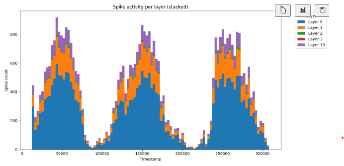
print(f"On chip inference accuracy: {correct_predictions/len(spiking_activity)}")Anaylse spiking activity through time
The layer 13 correspiond to the input data.
import pickle
from collections import Counter
import numpy as np
import matplotlib.pyplot as plt

print(f"Number of inferences: {len(spiking_activity)}")

inference_to_analyse = 0
print(f"Inference analysed: {inference_to_analyse}")

monitored_events = spiking_activity[inference_to_analyse]
print(f"Total number of events for the inference: {len(monitored_events)}")


# Extract timestamps and layers
timestamps = [e.timestamp for e in monitored_events]
layers = [e.layer for e in monitored_events]

# Get min and max timestamp
min_t, max_t = min(timestamps), max(timestamps)

# Create 100 bins equally spaced
bins = np.linspace(min_t, max_t, 101)  # 101 edges = 100 bins
bin_centers = (bins[:-1] + bins[1:]) / 2  # for x-axis

# Unique layers
unique_layers = sorted(set(layers))

# Count spikes per bin per layer
counts = np.zeros((len(unique_layers), len(bins)-1), dtype=int)
layer_to_idx = {layer: i for i, layer in enumerate(unique_layers)}

for e in monitored_events:
    bin_idx = np.searchsorted(bins, e.timestamp, side="right") - 1
    if 0 <= bin_idx < len(bins)-1:
        counts[layer_to_idx[e.layer], bin_idx] += 1

# Plot stacked bar chart
bottom = np.zeros(len(bins)-1)

plt.figure(figsize=(12, 6))
for i, layer in enumerate(unique_layers):
    plt.bar(bin_centers, counts[i],
            bottom=bottom,
            width=(bins[1] - bins[0]),  # bar width = bin size
            align="center",
            label=f"Layer {layer}")
    bottom += counts[i]

plt.xlabel("Timestamp")
plt.ylabel("Spike count")
plt.title("Spike activity per layer (stacked)")
plt.legend(title="Layer", bbox_to_anchor=(1.05, 1), loc='upper left')
plt.tight_layout()
plt.show()
This is the spiking activity for each layer when the model is trained.
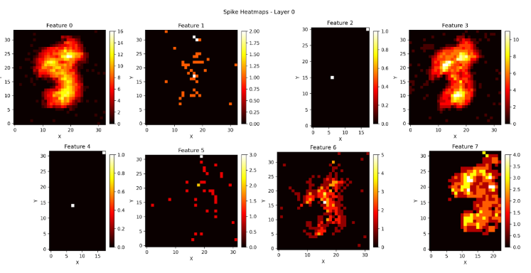
Analyse spiking activity through coordinates
import pickle
from collections import Counter
import numpy as np
import matplotlib.pyplot as plt
print(f"Number of inferences: {len(spiking_activity)}")
inference_to_analyse = 30
print(f"Inference analysed: {inference_to_analyse}")
events = spiking_activity[inference_to_analyse]
print(f"Total number of events for the inference: {len(events)}")
event_per_layer_count = Counter(event.layer for event in events)
layers_concerned = list(event_per_layer_count.keys())
print(f"Layers concerned: {layers_concerned}")
print(f"Number of events per layers: {dict(event_per_layer_count)}")
for layer_number in layers_concerned:
layer_events = [event for event in events if event.layer == layer_number]
num_features = max(e.feature for e in layer_events) + 1
# Prepare subplots
cols = min(num_features, 4) # up to 4 per row
rows = int(np.ceil(num_features / cols))
fig, axes = plt.subplots(rows, cols, figsize=(4*cols, 4*rows))
axes = np.atleast_2d(axes) # ensure 2D array for indexing
for feature in range(num_features):
filtered = [e for e in layer_events if e.feature == feature]
if filtered: # skip empty features
xs = [e.x for e in filtered]
ys = [e.y for e in filtered]
max_x, max_y = max(xs), max(ys)
heatmap = np.zeros((max_y + 1, max_x + 1), dtype=int)
for x, y in zip(xs, ys):
heatmap[y, x] += 1
else:
heatmap = np.zeros((1, 1)) # empty plot
ax = axes[feature // cols, feature % cols]
im = ax.imshow(heatmap, cmap='hot', origin='lower')
ax.set_title(f"Feature {feature}")
ax.set_xlabel("X")
ax.set_ylabel("Y")
fig.colorbar(im, ax=ax, fraction=0.046, pad=0.04)
# Remove unused subplots
for f in range(num_features, rows*cols):
fig.delaxes(axes[f // cols, f % cols])
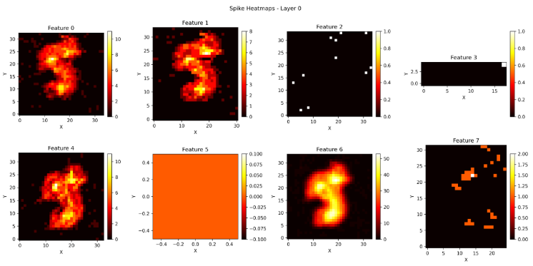
plt.suptitle(f"Spike Heatmaps - Layer {layer_number}")
plt.tight_layout()
plt.savefig(f"heatmaps_layer_{layer_number}.png", dpi=300)
plt.close()
print("Saved heatmaps as heatmaps_layer.png")This is the spiking activity of layer 0 when the model is untrained.
This is the spiking activity of layer 0 when the model is trained.
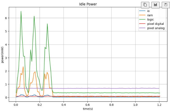
Analyse power consumption
inference_to_analyse = 0


import matplotlib.pyplot as plt
from collections import defaultdict

# Replace with your actual PowerMeasurement list
measurements = power_monitoring[inference_to_analyse]

# Channel names
p_track_name = ["io", "ram", "logic", "pixel digital", "pixel analog"]

# Group data by channel
data_by_channel = defaultdict(lambda: {"timestamps": [], "values": []})

for m in measurements:
    data_by_channel[m.channel]["timestamps"].append(m.timestamp/1e6)
    data_by_channel[m.channel]["values"].append(m.value* 1e3)

# Create plot
fig, ax = plt.subplots(figsize=(10, 6))

for channel, data in data_by_channel.items():
    label = p_track_name[channel] if channel < len(p_track_name) else f"Channel {channel}"
    ax.plot(data["timestamps"], data["values"], label=label)

ax.set_xlabel("time(s)")
ax.set_ylabel("power(mW)")
ax.set_title("Idle Power")
ax.legend(loc="upper right", fontsize=10)
ax.grid(True)

plt.show()
This is the power consumption when the model is trained.